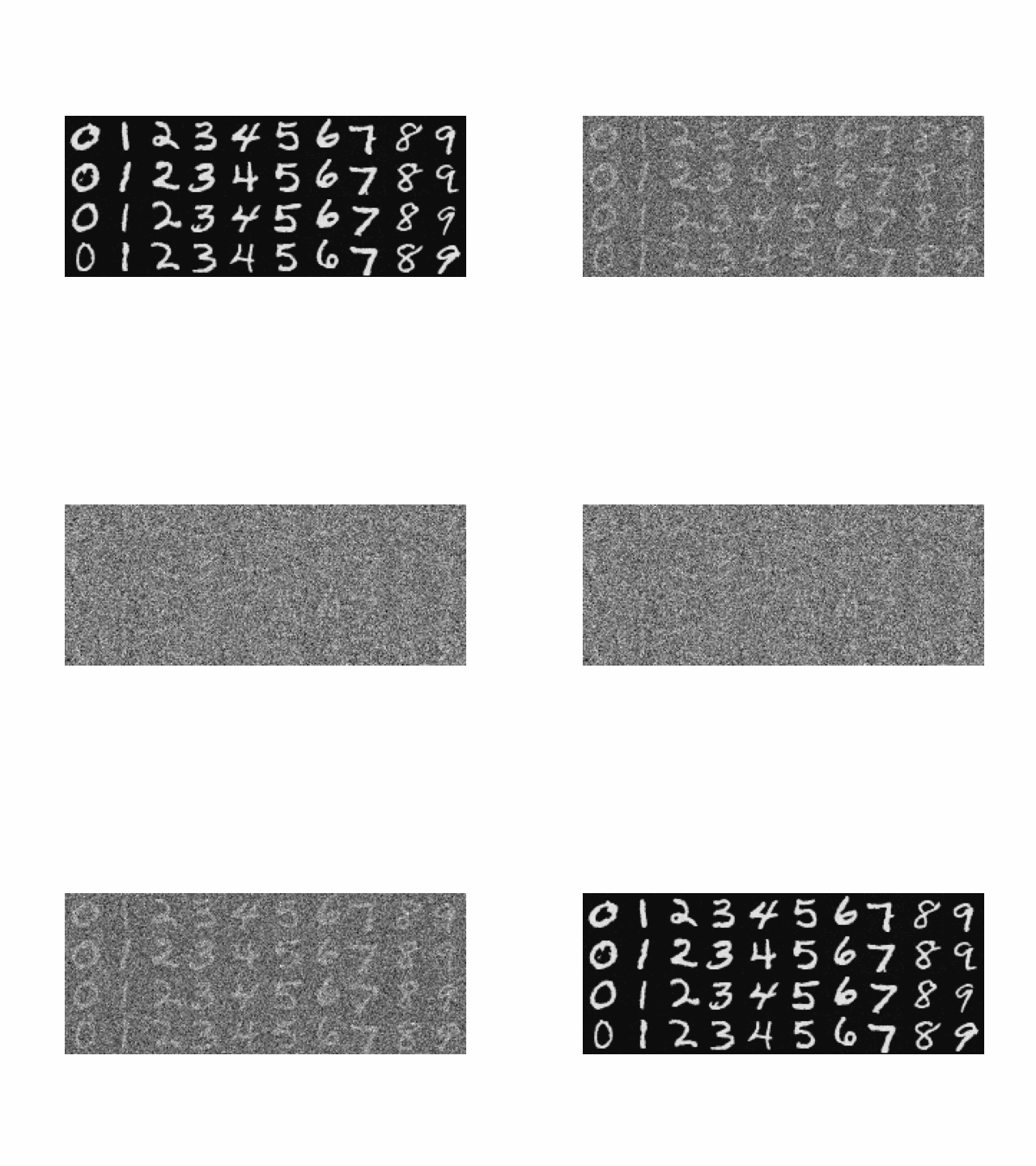
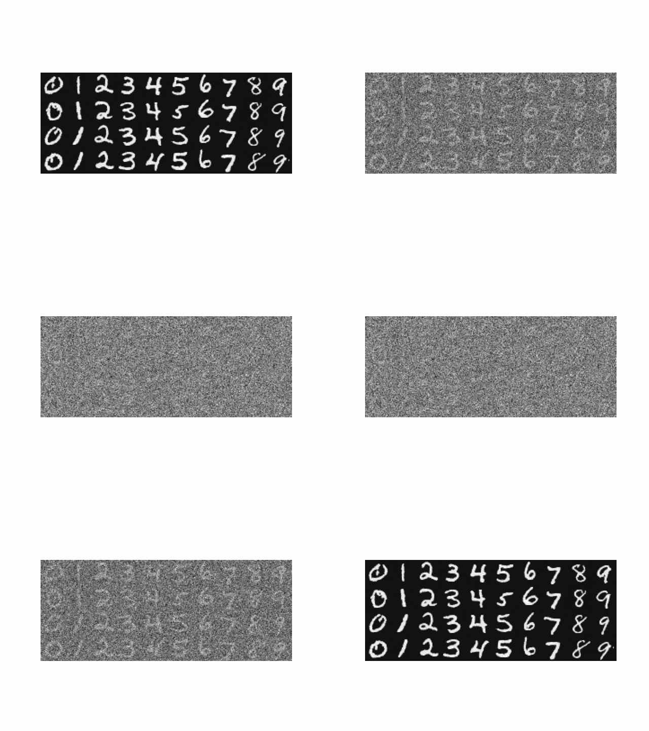
The power of Diffusion Models
Diffusion models are trained for denoising by estimating the noise in a given input. They are widely applicable in image denoising, as well as image generation.
In this project, we are using the DeepFloyd model by Huggingface.
Sampling from the Model
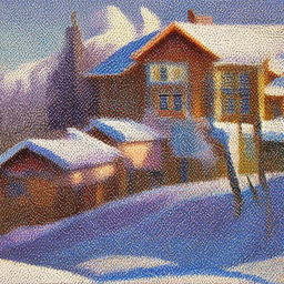
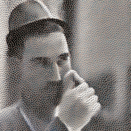
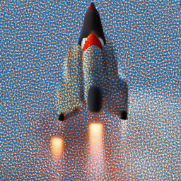
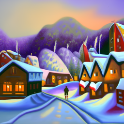
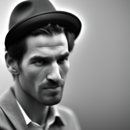
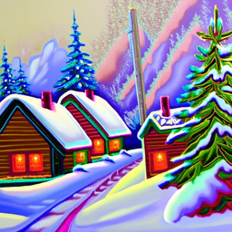
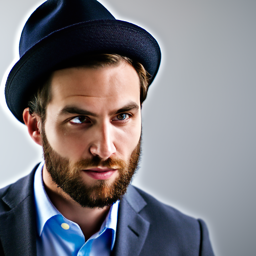
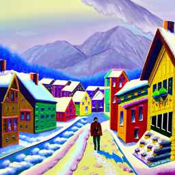
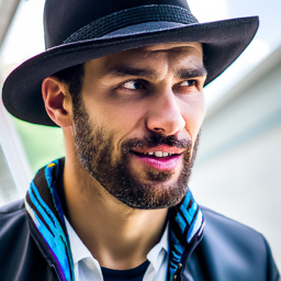
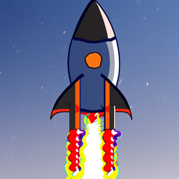
Here are some images generated using the following prompts with different number of inference steps. The random seed is selected to be 180.
| An oil painting of a snowy mountain village | A man wearing a hat | A rocket ship | |
|---|---|---|---|
| 5 inference steps |
|
|
|
| 10 inference steps |
|
|

|
| 20 inference steps |
|
|

|
| 40 inference steps |
|
|
|
Notice how the quality of the image increases as the number of inference steps increases, especially the details. Also, the images become more relevant to the text prompt and makes more sense in general with more inference steps.
Forward Process
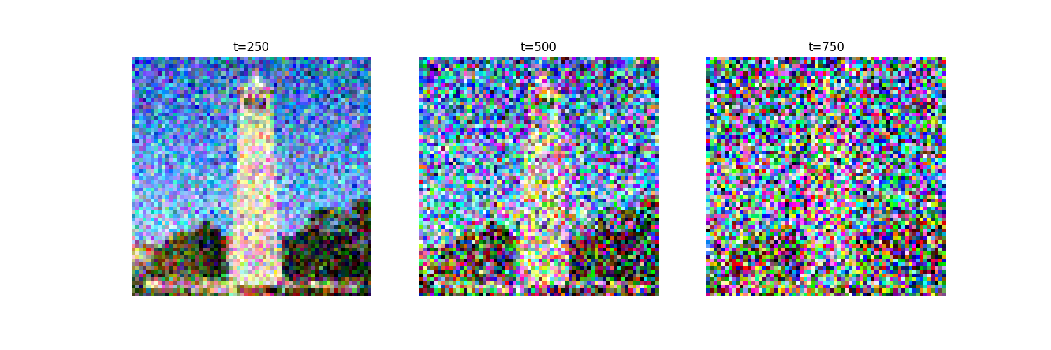
In the forward process, we take a clean image and gradually add noise to it. More specifically, we add a zero-mean, i.i.d. Gaussian noise to each pixel of the image. This is equivalent to computing $$x_t = \sqrt{\bar{\alpha}_t} x_0 + \sqrt{1 - \bar{\alpha}_t} \epsilon$$ where $\epsilon \sim \mathcal{N} (0, 1)$. In the DeepFloyd model, $T \in [0, 999]$.
We take an image of the Campanile as an example and show the noisy image at $T \in \{250, 500, 750\}$. This example shows that the image gradually becomes pure noise as $T$ increases.
Classical Denoising
Recall that a Gaussian filter removes the high-frequency components of an image. Since the Gaussian noise is of higher frequency than the elements in the original image, we can mitigate the noise by applying a Gaussian filter.
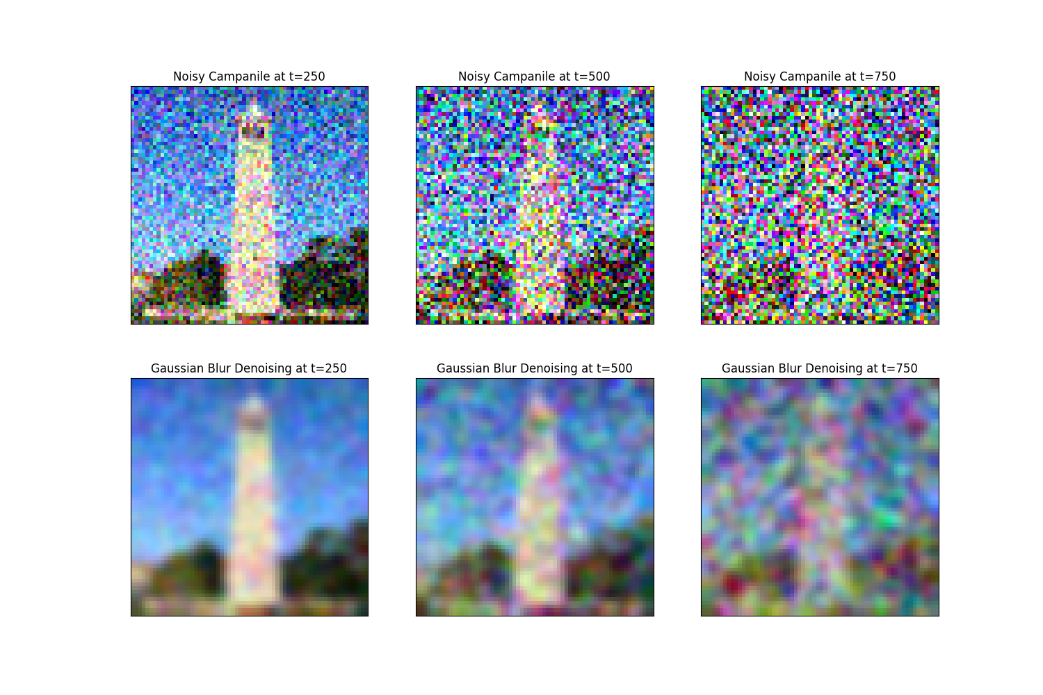
The result is clearly not ideal, especially for the cases with higher noise levels. This is because the Gaussian filter also caused loss of high-frequency information in the original image.
One-Step Denoising
Now, we use the pretrained diffusion model for the denoising task.
The DeepFloyd model is trained with both time conditioning and text conditioning, which takes
the time $T$ and a text embedding as a conditioning signal.
Here, we simply use the embedding a high quality photo as an "empty" prompt.
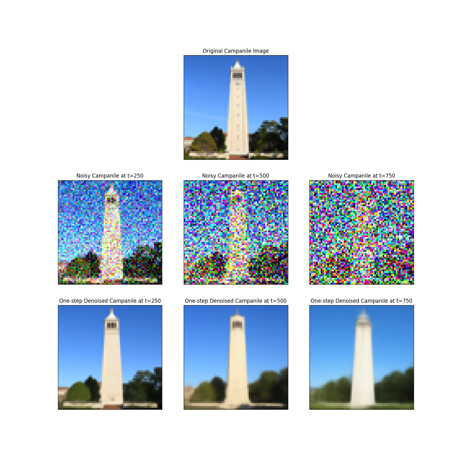
We apply the model at various time $T$ to estimate the noise in the image, and recover the clean image with the same formula as in the forward process.
The results are as follows. Notice that the model is also "editing" the image a little bit to create another version of Campanile that also makes sense.
Iterative Denoising
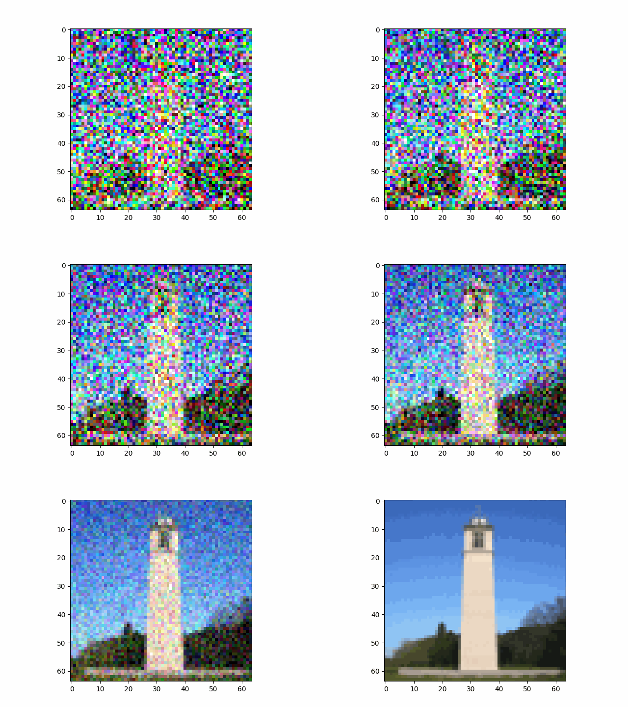
Although the one-step denoising did a reasonable job, the result is still not ideal when the image is especially noisy. However, note that diffusion models are trained to denoise the image iteratively. Instead of trying to remove all the noise in one step, we do the reverse of the forward process by removing the noise little by little.
In the iteration at time $t$, we use the one-step denoising to estimate the clean image $\hat{x}_0$ based the noisy image $x_t$ and the noise level at time $t$. Then, we get the estimation of the previous time-step by taking a linear combination of the noisy image, $$x_{t'} = \frac{\sqrt{\bar{\alpha}_{t'}} \beta_t}{1 - \bar{\alpha}_t}x_0 + \frac{\sqrt{\alpha_t} (1 - \bar{\alpha}_{t'})}{1 - \bar{\alpha}_t}x_t + v_\sigma$$ where $\bar{\alpha}_t$ is related to the noise schedule, which we will stick to the design choice behind the DeepFloyd model. $v_\sigma$ is the estimated variance to add back into the image.
Also, to speed up the process, it turns out we can skip some of the timesteps. Here, we use a strided timestep with step size 30.
The result of the iterative denoising is as follows. Compared side-by-side with the results of previous methods, the iterative denoising has by far the best performance.
| $t=90$ | $t=240$ | $t=390$ | $t=540$ | $t=690$ |
|---|---|---|---|---|

|

|

|

|

|
| Original | Iterative Denoised Campanile | One-step Denoised Campanile | Gaussian-Blurred Campanile |

|

|

|

|
Diffusion Model Sampling
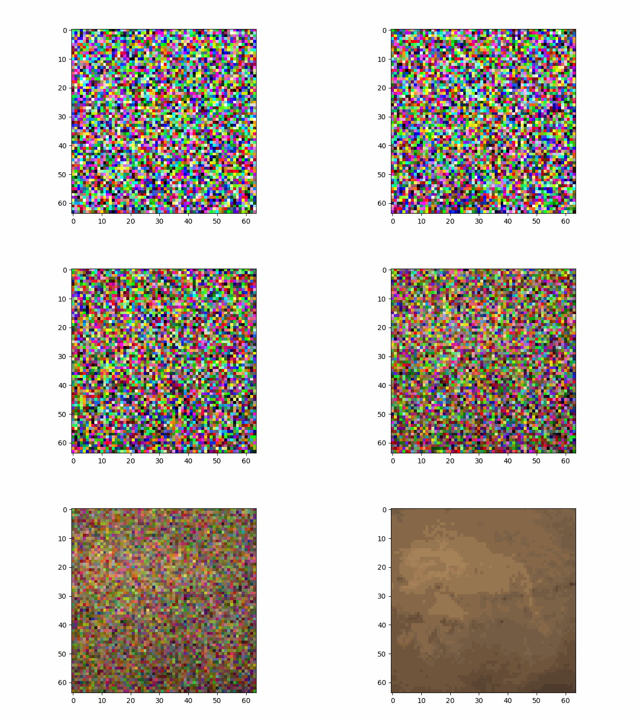
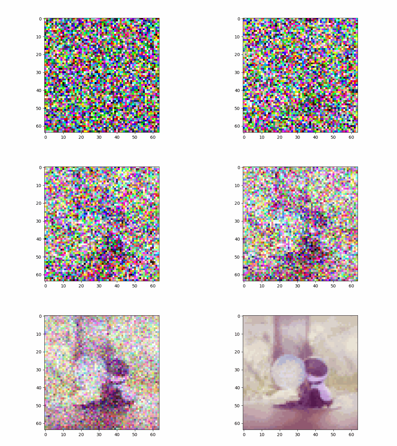
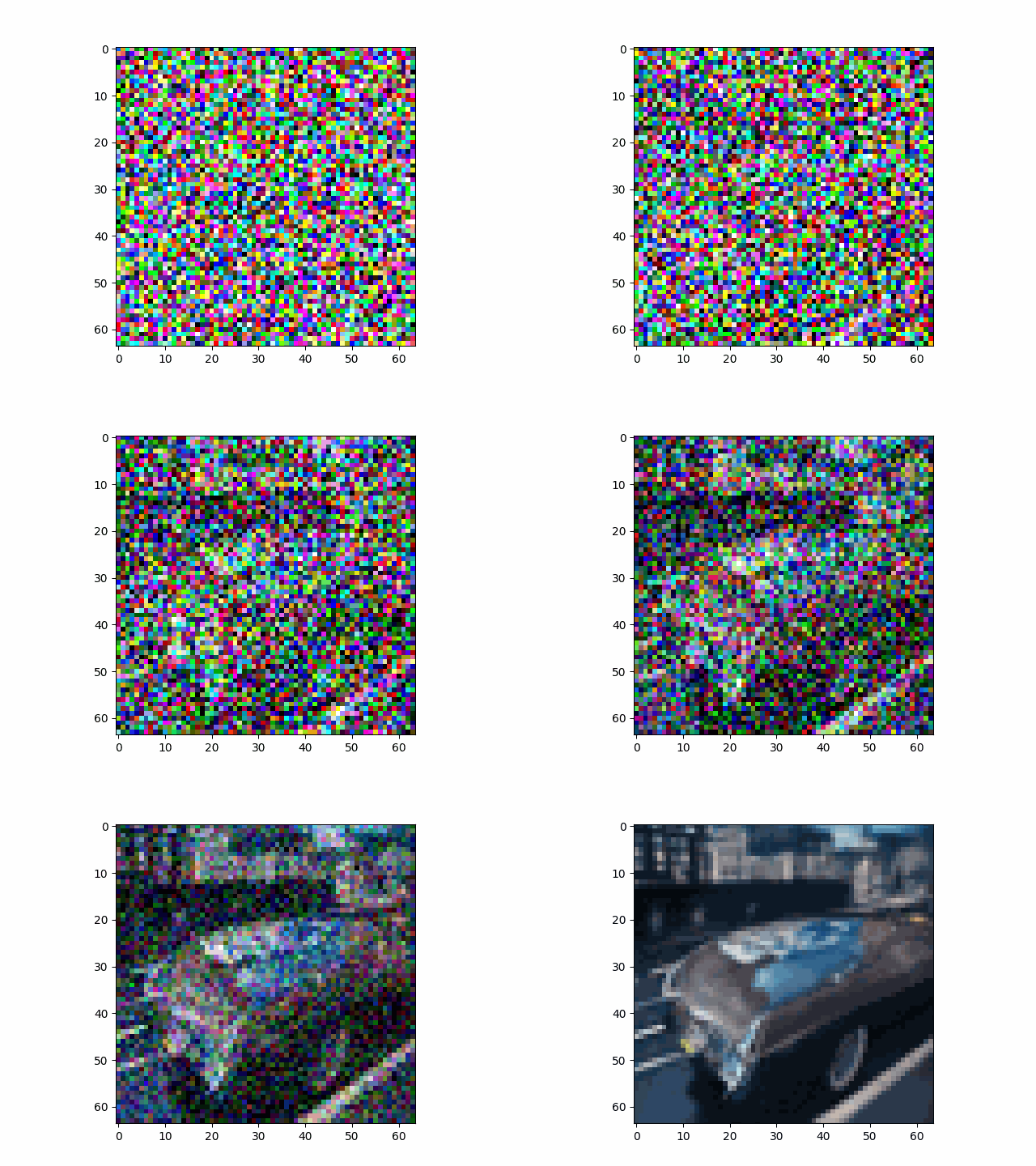
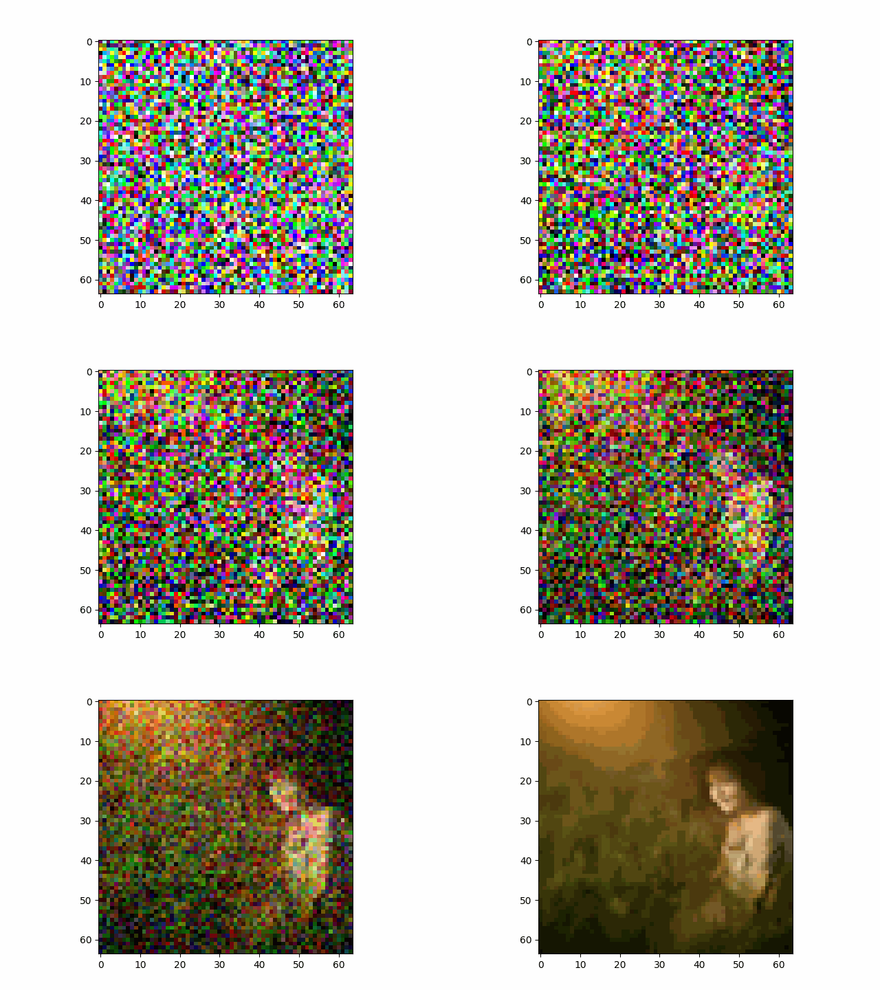
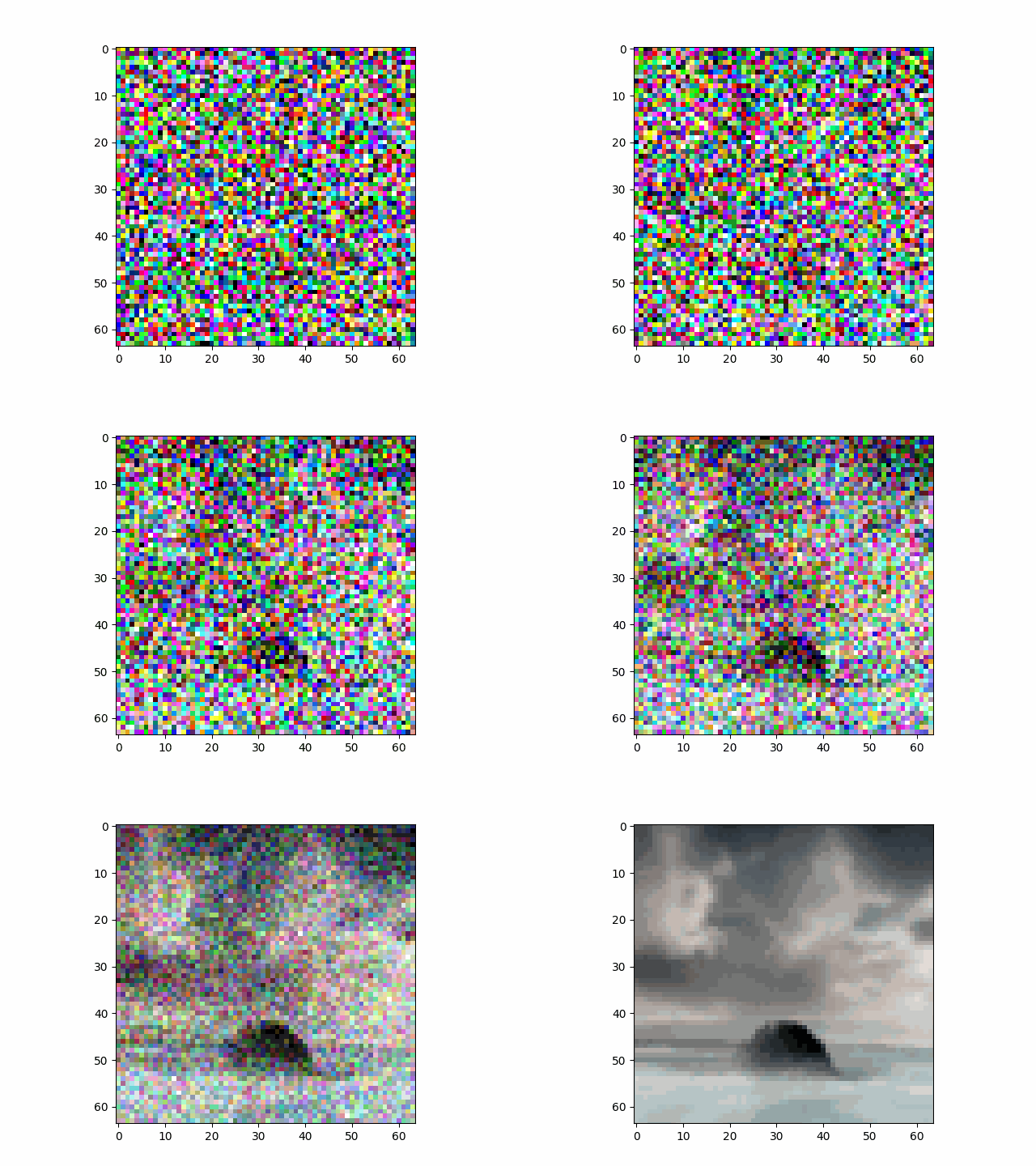
Similar to what we did in the beginning, we can also use the diffusion model to denoise an image that contains nothing but pure noise.
Below are some results.
| Sample 1 | Sample 2 | Sample 3 | Sample 4 | Sample 5 |
|---|---|---|---|---|
|
|
|
|
|
We can see that some of the images generated from pure noise are not so good.
Classifier-free Guidance
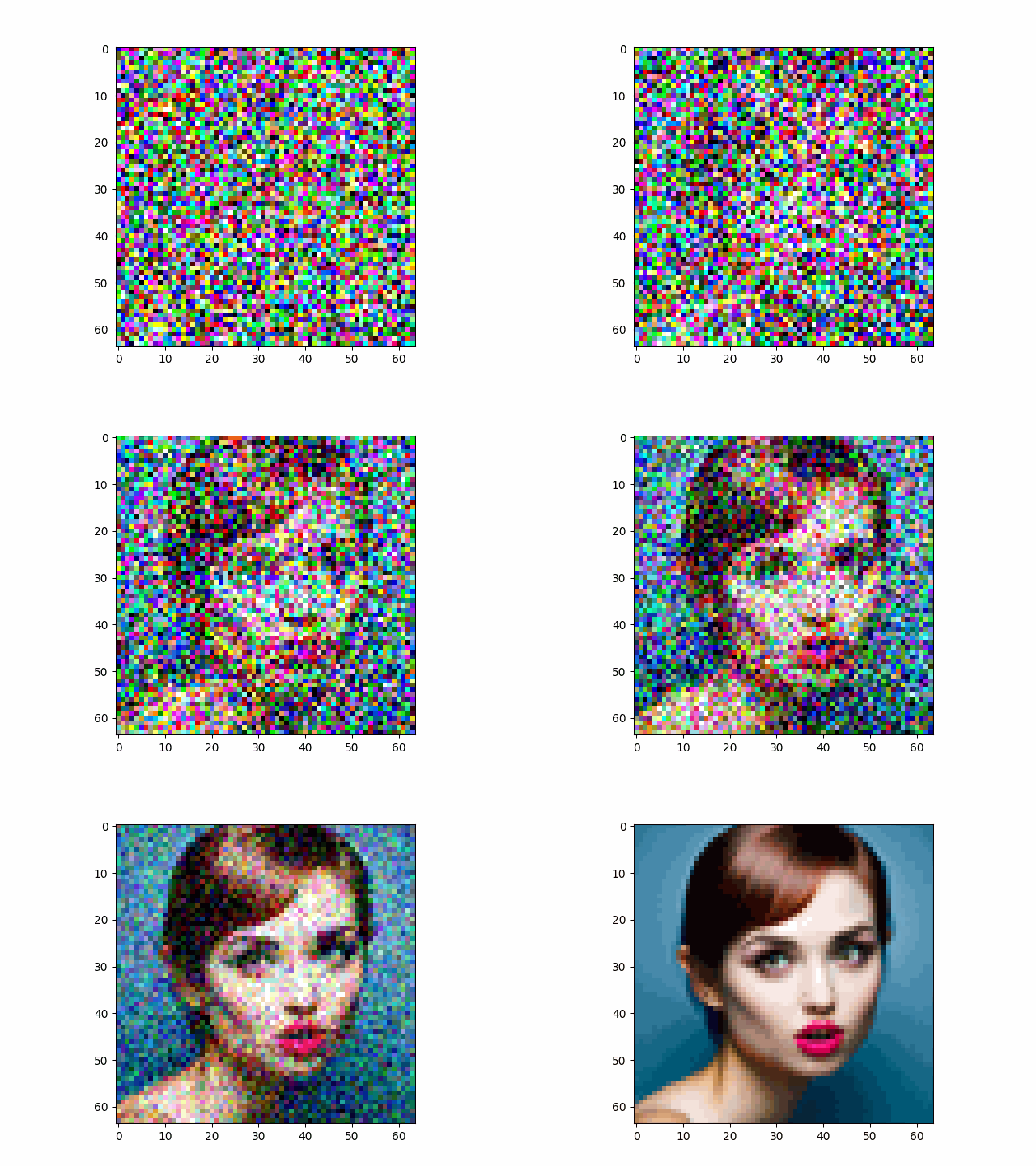
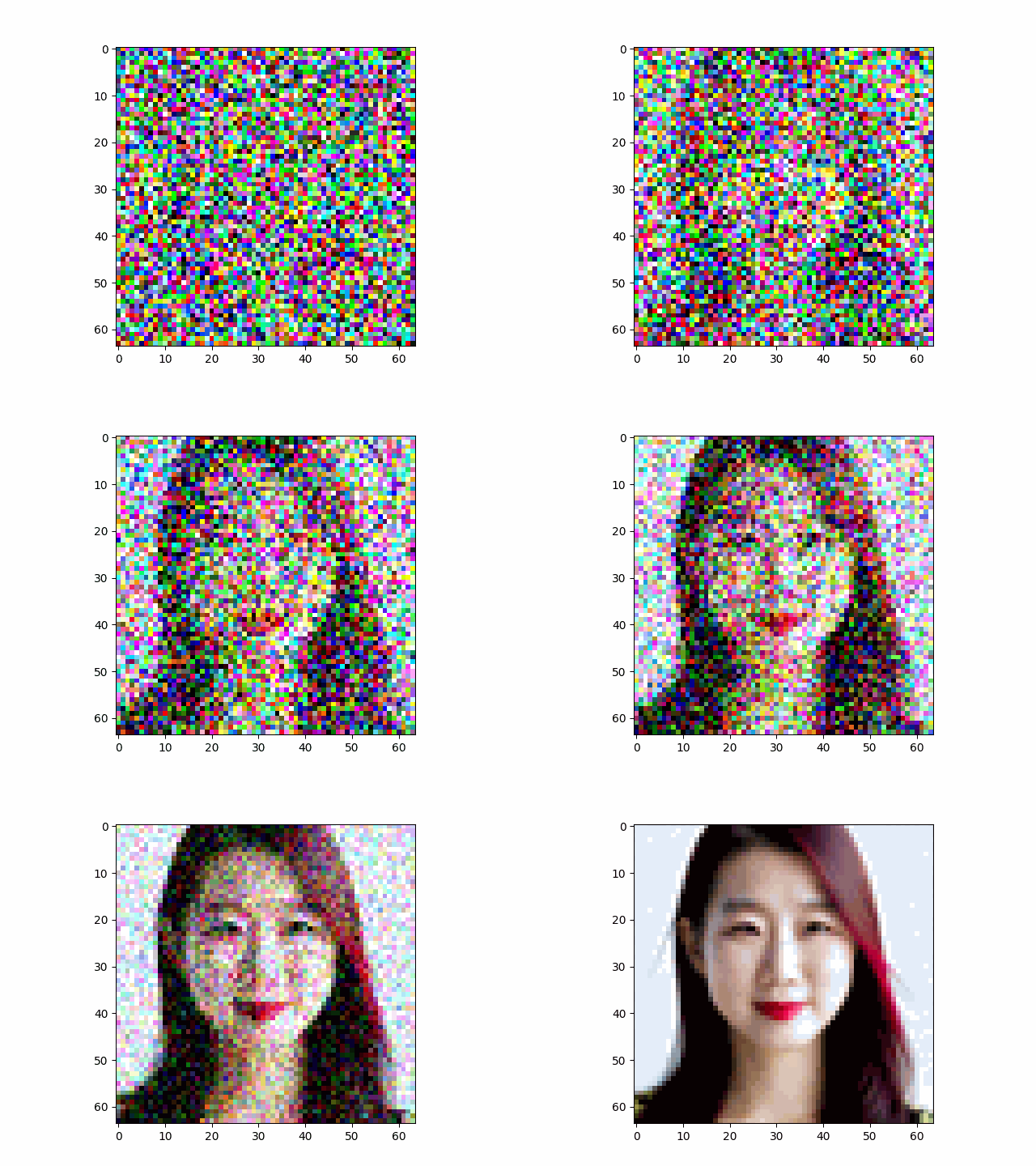
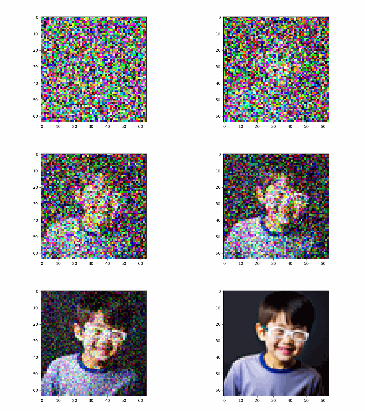
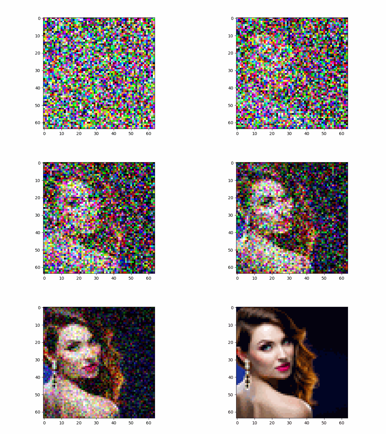
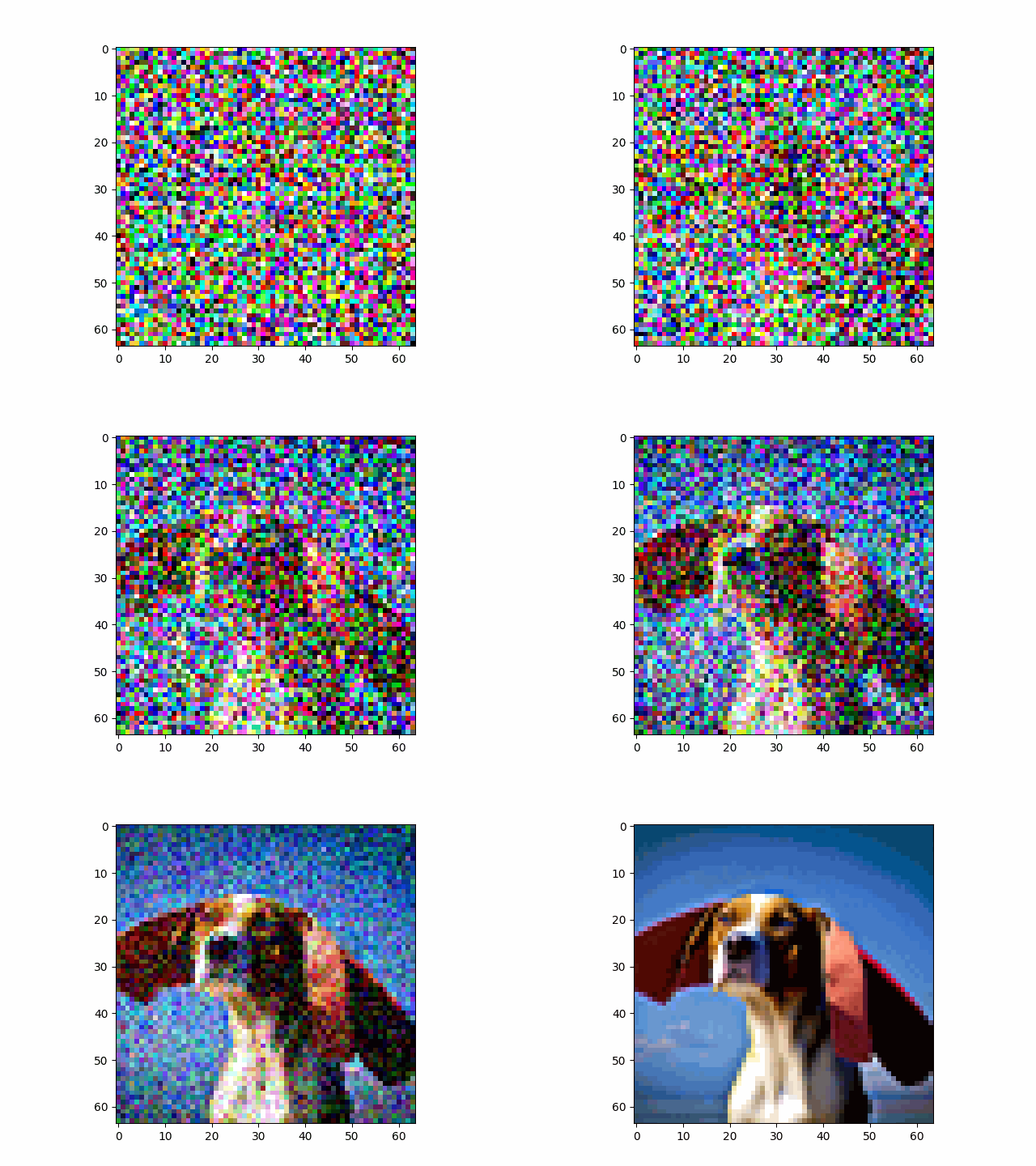
To improve the quality of the generated images, we borrow the idea from caricature generation. In each iteration of the denoising process, we additionally estimate the noise with a truly empty prompt, and "push" the image towards the "realistic" manifold, i.e., $$\epsilon = \epsilon_u + \gamma (\epsilon_c - \epsilon_u)$$ where $\epsilon_u$ is the estimated noise with an empty prompt, a.k.a. the unconditioned noise estimation, while $\epsilon_c$ is the noise estimated with our prompt, a.k.a. the conditioned noise estimation. This trick is known as Classifier-free Guidance (CFG), and its strength is controlled by the $\gamma$.
Below are some results generated with CFG.
| Sample 1 | Sample 2 | Sample 3 | Sample 4 | Sample 5 |
|---|---|---|---|---|
|
|
|
|
|
Image-to-Image Translation
As mentioned in the previous section, the denoiser doesn't usually revert the image back to its clean version, but performs some reasonable "editing" as well. Utilizing this fact, we can intentionally add some noise to the image and pass it into the diffusion model. This follows the SDEdit algorithm.
Here we inject different levels of noise into the campanile image, and here are the results. Not surprisingly, the larger the noise level, the more significant the edit.
| i_start=1 | i_start=3 | i_start=5 | i_start=7 | i_start=10 | i_start=20 |
|---|---|---|---|---|---|

|

|

|

|

|

|
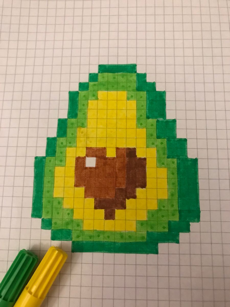
Editing Hand-Drawn and Web Images
Let's apply this on some other images we can find on the web.
| i_start=1 | i_start=3 | i_start=5 | i_start=7 | i_start=10 | i_start=20 | Original |
|---|---|---|---|---|---|---|

|

|

|

|

|

|
|
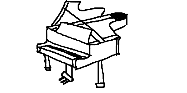
It is even possible to draw a sketch by hand and have it rendered into a realistic image. Here are some examples.
| i_start=1 | i_start=3 | i_start=5 | i_start=7 | i_start=10 | i_start=20 | Original |
|---|---|---|---|---|---|---|

|

|

|

|

|

|

|

|

|

|

|

|

|
|
Inpainting
We can also limit the editing to a specific region, following the idea in the InPainting paper. We define a binary mask with the same shape as the spatial dimensions of the image. In each iteration of CFG, we "force" the pixels outside the editing area to be the ground truth plus the correct amount of noise. In other words, $$x_t \gets \mathbb{m} x_t + (1 - \mathbb{m}) \mathrm{forward}(x_{orig}, t)$$ This maintains the correct noise level at each timestep, while ensuring only the editing area gets modified.
Below are some examples of the output of the InPainting algorithm.
| Original | Mask | Region to Edit | Result |
|---|---|---|---|

|

|

|
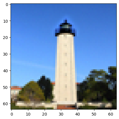
|

|

|

|

|

|

|

|

|
Text-Conditional Image-to-image Translation
So far, we've been only using the "empty" prompt a high quality photo.
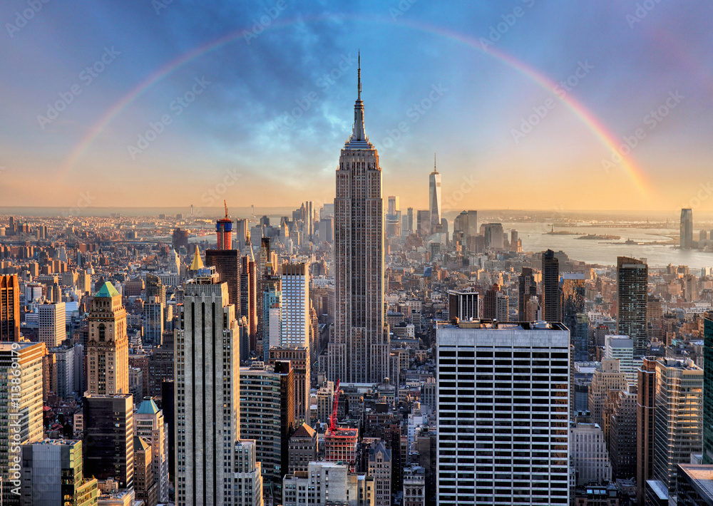
However, if the prompt contains specific descriptions, we can modify the content of the photo.
We adopt a similar algorithm as SEdit, but this time using various different prompts. Some examples of the results are shown below.
| Prompt | i_start=1 | i_start=3 | i_start=5 | i_start=7 | i_start=10 | i_start=20 | Original |
|---|---|---|---|---|---|---|---|
| a rocket ship |

|

|

|

|

|

|

|
| A violently erupting volcano |

|

|

|

|

|
 |
 |
| A tropical forest |

|

|

|

|

|

|
|
| A Steinway nine-foot grand piano |

|

|

|

|

|

|

|
Visual Anagrams
With the diffusion model, we can also create multi-view optical illusions with ideas from Visual Anagrams paper.
Starting from an image with pure noise, we run the denoising algorithm with the noisy image using the first prompt, and in the same time use a second prompt on the same image flipped up-side-down. The estimated noise at each timestep is the average of the two inferred noise. In other words, $$\epsilon_1 = \mathrm{UNet}(x_t, t, p_1)$$ $$\epsilon_2 = \mathrm{flip}(\mathrm{UNet}(\mathrm{flip}(x_t), t, p_2))$$ $$\epsilon = (\epsilon_1 + \epsilon_2) / 2$$
Below are some visual anagrams created using this algorithm. Hover on the image to rotate it upside down.

Upside-down: an oil painting of an old man

Upside down: an oil painting of a snowy mountain village

Upside down: a photo of a man
Hybrid Images
Another type of visual illusion are images that look different when viewed from up close and from afar. For this type of illusion, we implement the Factorized Diffusion. The algorithm is $$\epsilon_1 = \mathrm{UNet}(x_t, t, p_1)$$ $$\epsilon_2 = \mathrm{UNet}(x_t, t, p_2)$$ $$\epsilon = f_{\mathrm{lowpass}}(\epsilon_1) + f_{\mathrm{highpass}}(\epsilon_2)$$ where $f_{\mathrm{lowpass}}$ and $f_{\mathrm{highpass}}$ are low pass and high pass functions, respectively. Here, the low pass function is the Gaussian Blur with the kernel size of 33 and sigma of 2, and the high pass function is the Laplacian filter with the same kernel size and sigma. $p_1$ and $p_2$ are two different prompts for the hybrid image.
Below are some results.
| Hybrid image of a skull and a waterfall | Hybrid image of the Amalfi coast and people around a campfire | Hybrid image of a snowy mountain village and a dog |
|---|---|---|

|

|

|
